Asymmetric Delusions and Pragmatism

Sometimes I joke that to conservatives, the solution to every problem is to cut taxes; to liberals, the solution to every problem is to eat local.  Of course, purported panaceas on both the left and right are snake oil, even if peddled by true believers.

So, the other day I picked on my own tribe: foodies.  To be frank, I have a love-hate relationship with the movement.  It has thin and oftentimes paranoid underpinnings.  But while a lot of things advocated by the movement are illogical or scientifically baseless (like the dangers of GMOs), the movement also strikes me as mostly harmless, and sometimes even beneficial.  There are some important and disastrous exceptions, like the movement to kill golden rice, which could save the lives of millions and save millions more from blindness.

But for the most part, the movement to "eat local," and all it's offspring, doesn't strike me as particularly harmful.   Here in Hawai'i there are delusional ideas that we ought to stop importing food and go back to the traditional ways of living off taro.  Obviously this isn't going to happen.  Even though they banned GMOs on some of our islands, exceptions were made for key crops actually grown.  Still, the movement does seem to be strong enough to help protect cultural heritage, an important public good.  It also cultivates a food culture that breeds great restaurants and fresh local produce.  After all, wasn't the whole movement inspired by my former Berkeley neighbor, restaurant extraordinaire, Alice Waters? (I never met her, but lived two doors down, in an in-law studio during grad school)  The movement isn't going to save the planet or feed the world, but it sure makes my privileged little world a lot nicer and a little healthier.

What about delusions on the right?  Front and center would be climate change denialism.  Not far behind would be anti-Keynesianism, or the austerity movement.  As Paul Krugman reminds us every day, quite persuasively in my view, these delusions have hardly been harmless.  And in contrast to foodies, the radical right has a whole lot of power, controlling both houses of Congress and rich backing by Wall Street, the Koch brothers and friends.

So, while reasoning and herd behavior on both extremes seems equally delusional at times, the delusional right strikes me as more destructive and much more powerful.

But then, speaking honestly, I identify more with the left than the right.  So am I being too soft on the lefties?  I don't think so, but feel free to weigh in. I think the lefty culture tends to be a bit more introspective by nature than the right.  The right doesn't tend to tease their own quite like I did the other day, not without swift excommunication.  And I think lefties, by their nature, are a little bit more susceptible to evidence and persuasion.  They also, by nature, possess visceral independence and eschew the party line.  Maybe that's what I was doing the other day.

Given the real political asymmetry here, I do feel a little guilty for picking on foodies.  But not too much.  I don't really want to go out and do a lot of research on the topic of food waste to prove how silly this stuff is, or to prove that while GMOs can have some undesirable side effects they aren't Frankenfoods. For the most part this is a fight that isn't worth fighting.  I figure it's better to focus on the things that really do matter.

But I figured it was worth a blog post, because I think we all do better when we eschew our innate tendency toward tribalism, try to figure out what's really going on, and find the most pragmatic solutions to real problems.

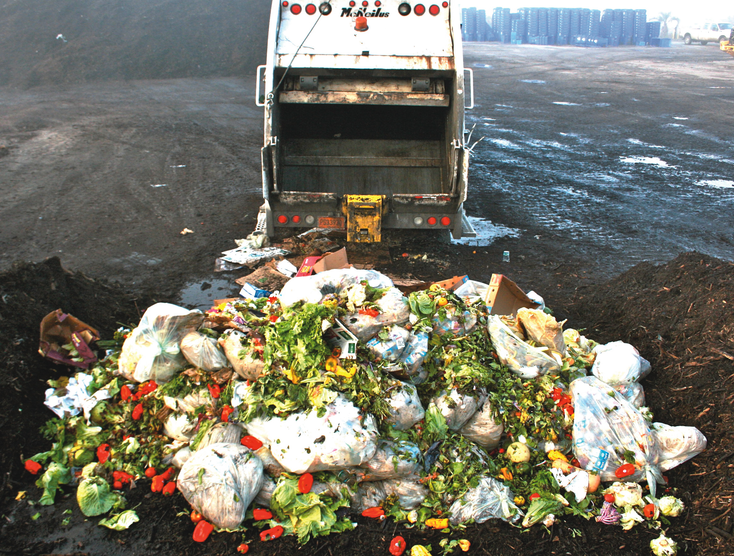
Food Waste Delusions

A couple months ago the New York Times convened a conference "Food for Tomorrow: Farm Better. Eat Better. Feed the World."  Keynotes predictably included Mark Bittman and Michael Pollan.  It featured many food movement activists, famous chefs, and a whole lot of journalists. Folks talked about how we need to farm more sustainably, waste less food, eat more healthfully and get policies in place that stop subsidizing unhealthy food and instead subsidize healthy food like broccoli.

Sounds good, yes? If you're reading this, I gather you're familiar with the usual refrain of the food movement.  They rail against GMOs, large farms, processed foods, horrid conditions in confined livestock operations, and so on.  They rally in favor of small local farms who grow food organically, free-range antibiotic free livestock, diversified farms, etc.  These are yuppies who, like me, like to shop at Whole Foods and frequent farmers' markets.  

This has been a remarkably successful movement.  I love how easy it has become to find healthy good eats, bread with whole grains and less sugar, and the incredible variety and quality of fresh herbs, fruits, vegetables and meat.  Whole Paycheck Foods Market has proliferated and profited wildly.  Even Walmart is getting into the organic business, putting some competitive pressure on Whole Foods. (Shhhh! --organic isn't necessarily what people might think it is.)

This is all great stuff for rich people like us. And, of course, profits.  It's good for Bittman's and Pollan's book sales and speaking engagements.  But is any of this really helping to change the way food is produced and consumed by the world's 99%?  Is it making the world greener or more sustainable?  Will any of it help to feed the world in the face of climate change?

Um, no.  

Sadly, there were few experts in attendance that could shed scientific or pragmatic light on the issues.  And not a single economist or true policy wonk in sight. Come on guys, couldn't you have at least invited Ezra Klein or Brad Plummer?  These foodie journalists at least have some sense of incentives and policy. Better, of course, would be to have some real agricultural economists who actually know something about large-scale food production and policies around the world. Yeah, I know: BORING!

About agricultural polices: there are a lot of really bad ones, and replacing them with good policies might help.  But a lot less than you might think from listening to foodies.  And, um, we do subsidize broccoli and other vegetables, fruits, and nuts.  Just look at the water projects in the West. 

Let me briefly take on one issue du jour: food waste.  We throw away a heck of a lot of food in this country, even more than in other developed countries.  Why?  I'd argue that it's because food is incredibly cheap in this country relative to our incomes.  We are the world's bread basket.  No place can match California productivity in fruit, vegetables and nuts.  And no place can match the Midwest's productivity in grains and legumes.  All of this comes from remarkable coincidence of climate, geography and soils, combined with sophisticated technology and gigantic (subsidized) canal and irrigation systems in the West.  

Oh, we're fairly rich too.  

Put these two things together and, despite our waste, we consume more while spending less on food than any other country.  Isn't that a good thing?  Europeans presumably waste (a little) less because food is more scarce there, so people are more careful and less picky about what they eat. Maybe it isn't a coincidence that they're skinnier, too.

What to do? 

First, it's important to realize that there are benefits to food waste.  It basically means we get to eat very high quality food and can almost always find what we want where and when we want it.  That quality and convenience comes at a cost of waste.  That's what people are willing to pay for.  

If anything, the foodism probably accentuates preference for high quality, which in turn probably increases waste.  The food I see Mark Bittman prepare is absolutely lovely, and that's what I want.  Don't you?

Second, let's suppose we implemented a policy that would somehow eliminate a large portion of the waste.  What would happen?  Well, this would increase the supply of food even more.  And sinse we have so much already, and demand for food is very inelastic, prices would fall even lower than they are already.  And the temptation to substitute toward higher quality--and thus waste more food--would be greater still.  

Could the right policies help?  Well, maybe.  A little. The important thing here is to have a goal besides simply eliminating waste.  Waste itself isn't problem. It's not an externality like pollution.  That goal might be providing food for homeless or low income families.  Modest incentive payments plus tax breaks might entice more restaurants, grocery stores and others to give food that might be thrown out to people would benefit from it.  This kind of thing happens already and it probably could be done on a larger scale. Even so, we're still going to have a lot of waste, and that's not all bad. 

What about correcting the bad policies already in place?  Well, water projects in the West are mainly sunk costs.  That happened a long time ago, and water rights, as twisted as they may be, are more or less cemented in the complex legal history.   Today, traditional commodity program support mostly takes the form of subsidized crop insurance, which is likely causing some problems.  The biggest distortions could likely be corrected with simple, thoughtful policy tweaks, like charging higher insurance premiums to farmers who plant corn after corn instead of corn after soybeans.  But mostly it just hands cash (unjustly, perhaps) to farmers and landowners.  The odds that politicians will stop handing cash to farmers is about as likely as Senator James Inhofe embracing a huge carbon tax.  Not gonna happen.

But don't worry too much.  If food really does get scarce and prices spike, waste will diminish, because poorer hungry people will be less picky about what they eat.

Sorry for being so hard on the foodies.  While hearts and forks are in the right places, obviously I think most everything they say and write is naive.  Still, I think the movement might actually do some good.  I like to see people interested in food and paying more attention to agriculture.  Of course I like all the good eats.  And I think there are some almost reasonable things being said about what's healthy and not (sugar and too much red meat are bad), even if what's healthy has little to do with any coherent strategy for improving environmental quality or feeding the world.  

But perhaps the way to change things is to first get everyones' attention, and I think foodies are doing that better than I ever could.

The Hottest Year on Record, But Not in the Corn Belt

Here's Justin Gillis in his usual fine reporting of climate issues, and the map below from NOAA, via the New York Times.

Note the "warming hole" over the Eastern U.S., especially the upper Midwest, the all important corn belt region.  We had a bumper crop this year, and that's because while most of the world was remarkably warm, the corn belt was remarkably cool, especially in summer.

Should we expect the good fortune to continue?  I honestly don't know...

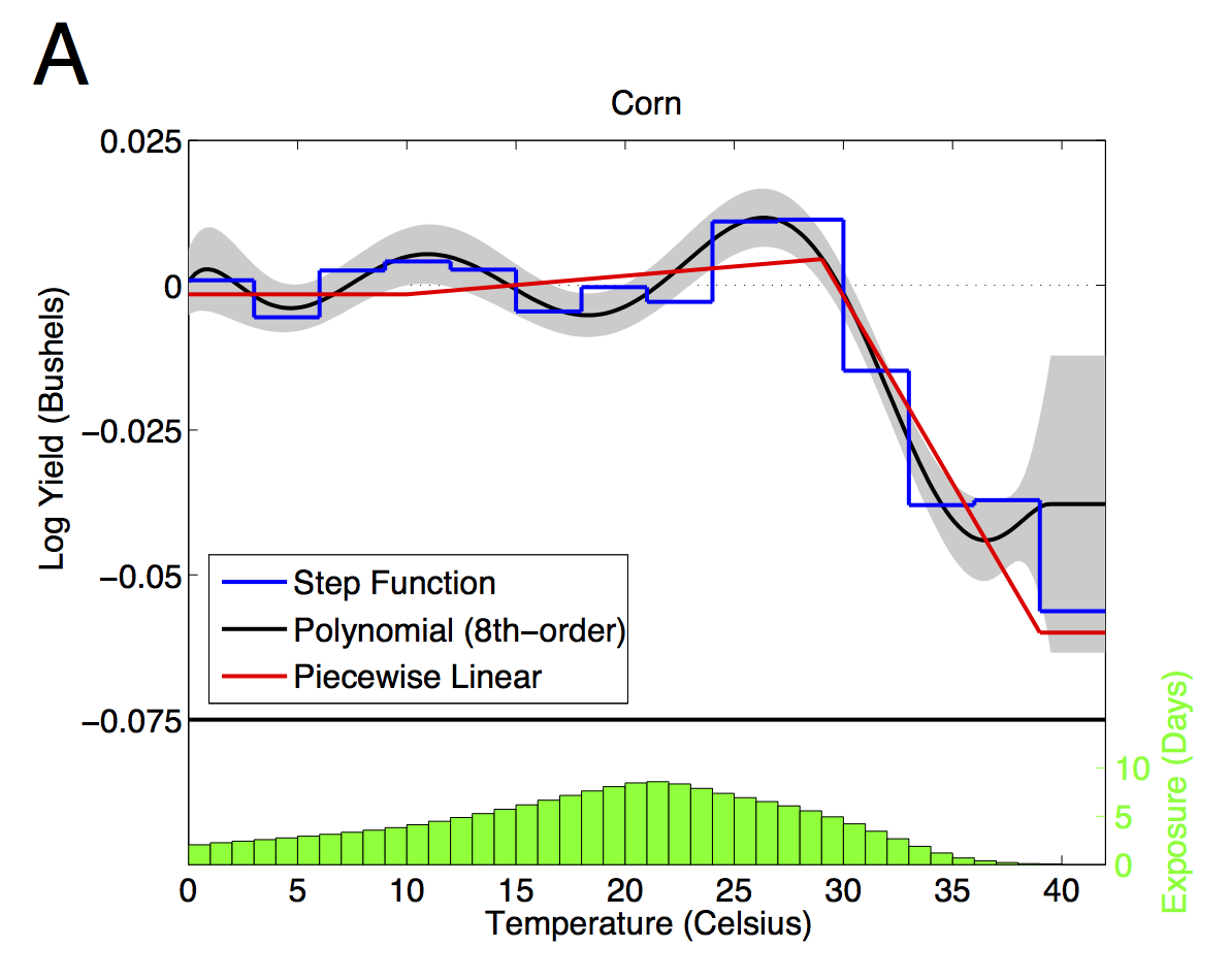
Searching for critical thresholds in temperature effects

Update 2: Okay, I think it's fixed.

Update: I just realized the code posted badly.  I don't know why.  It looks good in the cross-post at G-FEED.  I'll try to fix.

If google scholar is any guide, my 2009 paper with Wolfram Schlenker on the nonlinear effects of temperature on crop outcomes has had more impact than anything else I've been involved with.

A funny thing about that paper: Many reference it, and often claim that they are using techniques that follow that paper.  But in the end, as far as I can tell, very few seem to actually have read through the finer details of that paper or try to implement the techniques in other settings.  Granted, people have done similar things that seem inspired by that paper, but not quite the same.  Either our explication was too ambiguous or people don't have the patience to fully carry out the technique, so they take shortcuts.  Here I'm going to try to make it easier for folks to do the real thing.

So, how does one go about estimating the relationship plotted in the graph above?

Here's the essential idea:  averaging temperatures over time or space can dilute or obscure the effect of extremes.  Still, we need to aggregate, because outcomes are not measured continuously over time and space.  In agriculture, we have annual yields at the county or larger geographic level.  So, there are two essential pieces: (1) estimating the full distribution of temperatures of exposure (crops, people, or whatever) and (2) fitting a curve through the whole distribution.

The first step involves constructing the distribution of weather. This was most of the hard work in that paper, but it has since become easier, in part because finely gridded daily weather is available (see PRISM) and in part because Wolfram has made some STATA code available.  Here I'm going to supplement Wolfram's code with a little bit of R code.  Maybe the other G-FEEDers can chime in and explain how to do this stuff more easily.

First step:  find some daily, gridded weather data.  The finer scale the better.  But keep in mind that data errors can cause serious attenuation bias.  For the lower 48 since 1981, the PRISM data above is very good.  Otherwise, you might have to do your own interpolation between weather stations.  If you do this, you'll want to take some care in dealing with moving weather stations, elevation and microclimatic variations.  Even better, cross-validate interpolation techniques by leaving one weather station out at a time and seeing how well the method works. Knowing the size of the measurement error can also help correcting bias.  Almost no one does this, probably because it's very time consuming... Measurement error in weather data creates very serious problems (see here and here)

Second step:  estimate the distribution of temperatures over time and space from the gridded daily weather.  There are a few ways of doing this.  We've typically fit a sine curve between the minimum and maximum temperatures to approximate the time at each degree in each day in each grid, and then aggregate over grids in a county and over all days in the growing season.  Here are a couple R functions to help you do this:

# This function estimates time (in days) when temperature is
# between t0 and t1 using sine curve interpolation.  tMin and
# tMax are vectors of day minimum and maximum temperatures over
# range of interest.  The sum of time in the interval is returned.
# noGrids is number of grids in area aggregated, each of which 
# should have exactly the same number of days in tMin and tMax
 
days.in.range <- span=""> function( t0, t1 , tMin, tMax, noGrids )  {
  n   =  length(tMin)
  t0  =  rep(t0, n)
  t1  =  rep(t1, n)
  t0[t0 < tMin]   =  tMin[t0 < tMin]
  t1[t1 > tMax]  =  tMax[t1 > tMax]
  u  =  function(z, ind) (z[ind] - tMin[ind])/(tMax[ind] - tMin[ind])  
  outside  =  t0 > tMax | t1 < tMin
  inside  =  !outside
  time.at.range  =  ( 2/pi )*( asin(u(t1,inside)) - asin(u(t0,inside)) ) 
  return( sum(time.at.range)/noGrids ) 
}
 
# This function calculates all 1-degree temperature intervals for 
# a given row (fips-year combination).  Note that nested objects
# must be defined in the outer environment.
aFipsYear  =  function(z){
  afips   = Trows$fips[z]
  ayear    = Trows$year[z]
  tempDat  = w[ w$fips == afips & w$year==ayear, ]
  Tvect = c()
  for ( k in 1:nT ) Tvect[k] = days.in.range(
              t0   = T[k]-0.5, 
              t1   = T[k]+0.5, 
              tMin = tempDat$tMin, 
              tMax = tempDat$tMax,
              noGrids = length( unique(tempDat$gridNumber) )
              )
  Tvect
}

The first function estimates time in a temperature interval using the sine curve method.  The second function calls the first function, looping through a bunch of 1-degree temperature intervals, defined outside the function.  A nice thing about R is that you can be sloppy and write functions like this that use objects defined outside of the environment. A nice thing about writing the function this way is that it's amenable to easy parallel processing (look up 'foreach' and 'doParallel' packages).

Here are the objects defined outside the second function:

w       # weather data that includes a "fips" county ID, "gridNumber", "tMin" and "tMax".
        #   rows of w span all days, fips, years and grids being aggregated
 
tempDat #  pulls the particular fips/year of w being aggregated.
Trows   # = expand.grid( fips.index, year.index ), rows span the aggregated data set
T       # a vector of integer temperatures.  I'm approximating the distribution with 
        #   the time in each degree in the index T

To build a dataset call the second function above for each fips-year in Trows and rbind the results.

Third step:  To estimate a smooth function through the whole distribution of temperatures, you simply need to choose your functional form, linearize it, and then cross-multiply the design matrix with the temperature distribution.  For example, suppose you want to fit a cubic polynomial and your temperature bins that run from from 0 to 45 C.  The design matrix would be:

D = [    0          0          0   
            1          1           1
            2          4           8
             ...
           45     2025    91125]

These days, you might want to do something fancier than a basic polynomial, say a spline. It's up to you.  I really like restricted cubic splines, although they can over smooth around sharp kinks, which we may have in this case. We have found piecewise linear works best for predicting out of sample (hence all of our references to degree days).  If you want something really flexible, just make D and identity matrix, which effectively becomes a dummy variable for each temperature bin (the step function in the figure).  Whatever you choose, you will have a (T x K) design matrix, with K being the number of parameters in your functional form and T=46 (in this case) temperature bins. 

To get your covariates for your regression, simply cross multiply D by your frequency distribution.  Here's a simple example with restricted cubic splines:

library(Hmisc)
DMat = rcspline.eval(0:45)
XMat = as.matrix(TemperatureData[,3:48])%*%DMat
fit  = lm(yield~XMat, data=regData)
summary(fit)

Note that regData has the crop outcomes.  Also note that we generally include other covariates, like total precipitation during the season,  county fixed effects, time trends, etc.  All of that is pretty standard.  I'm leaving that out to focus on the nonlinear temperature bit. 

Anyway, I think this is a cool and fairly simple technique, even if some of the data management can be cumbersome.  I hope more people use it instead of just fitting to shares of days with each maximum or mean temperature, which is what most people following our work tend to do.  

In the end, all of this detail probably doesn't make a huge difference for predictions.  But it can make estimates more precise, and confidence intervals stronger.  And I think that precision also helps in pinning down mechanisms.  For example, I think this precision helped us to figure out that VPD and associated drought was a key factor underlying observed effects of extreme heat.

Agricultural Economics gets Politico

Update: For the record, I'm actually not against Federal crop insurance.  Like Obamacare, I generally favor it.  But the subsidies are surely much larger than they need to be for maximum efficiency.  And I think premiums could likely be better matched to risk, and that such adjustments would be good for both taxpayers and the environment.



Wow.  Frumpy agricultural economics goes Politico!

Actually, it's kind of strange to see a supposedly scandalous article in Politico in which you know almost every person mentioned. 

At issue is the federal crop insurance program.  The program has been around a long time, but its scope and size--the range crops and livestock insurable under the program and the degree to which taxpayers subsidize premiums--have grown tremendously over the last 20 years.  And the latest farm bill expands the program and its subsidies to grand new heights.

Nearly all the agricultural economists I know regard the crop insurance program (aka Obamacare for the corn) as overly subsidized.  But the issue here is not the subsides but the huge contracts received by agricultural economists moonlighting as well-paid consultants for USDA's Risk Management Agency (RMA), to help RMA design and run the insurance program.

For full disclosure: I used to work for USDA in the Economic Research Service and did some research on crop insurance.  Although, strangely, ties between ERS and RMA are thin to nonexistent. I've met and spoke to both Joe Glauber (USDA's Chief Economist) and Bruce Babcock (a leading professor of agricultural economics at Iowa State) a few times, and know and respect their work. And I used to work at NC State as a colleague of Barry Goodwin's.  I also went to Montana State for a master's degree way back, where I took courses from Myles Watts and Joe Attwood, who are mentioned in the article. I know Vince Smith from that time too.

Perhaps most importantly, some of my recent research uses some rich data resources that we obtained from RMA. But I have never received any monies from RMA.  Believe it or not, my interest is in the science, and despite having no vested financial interest in any of it, I have found myself in the cross hairs of agricultural interests who didn't seem to like my research findings.  Anyway, ag econ is a small, small world...

Okay, disclosures out of the way: What's the big deal here?  So ag economists work for RMA, make some nice cash, and then moonlight for the American Enterprise Institute to bash agricultural subsidies.  Yeah, there are are conflicts of interest, but it would seem that there are interests on many sides and the opportunistic ag economists in question seem willing to work for all of them.  They'll help RMA design crop insurance programs, but that doesn't mean they advocate for the programs or the level of subsidies farmers, insurance companies and program managers receive under them.  We observe the opposite.

I've got some sense of the people involved and their politics.  Most of them are pretty hard-core conservative (Babcock may be an exception, not sure), and my sense is that most are unsupportive of agricultural subsidies in general.  But none are going to turn down big pay check to try to make the program as efficient as possible.  I don't see a scandal here.  Really.

Except, I do kind of wonder why all this money is going to Illinois, Texas and Montana when folks at Columbia, Hawai'i, and Stanford could, almost surely, do a much better job for a fraction of  taxpayers' cost.  With all due respect (and requisite academic modesty--tongue in cheek), I know these guy's work, and I'm confident folks here at G-FEED could do a much better job.  I personally don't need a penny (okay, twist my arm and I'll take a month of summer salary). Just fund a few graduate students and let us use the data for good science.

 

Commodity Prices: Financialization or Supply and Demand?

I've often panned the idea that commodity prices have been greatly influenced by so-called financialization---the emergence of tradable commodity price indices and growing participation by Wall Street in commodity futures trading. No, Goldman Sachs did not cause the food and oil-price spikes in recent years. I've had good company in this view.   See, for example, Killian, Knittel and Pindyck, Krugman (also here), Hamilton, Irwin and coauthers, and I expect many others.

I don't deny that Wall Street has gotten deeper into the commodity game, a trend that many connect to  Gorton and Rouwenhorst (and much earlier similar findings).  But my sense is that commodity prices derive from more-or-less fundamental factors--supply and demand--and fairly reasonable expectations about future supply and demand.  Bubbles can happen in commodities, but mainly when there is poor information about supply, demand, trade and inventories.  Consider rice, circa 2008.

But most aren't thinking about rice. They're thinking about oil.

The financialization/speculation meme hasn't gone away, and now bigger guns are entering the fray, with some new theorizing and evidence.

Xiong theorizes (also see Cheng and Xiong and Tang and Xiong) that commodity demand might be upward sloping.  A tacit implication is that new speculation of higher prices could feed higher demand, leading to even higher prices, and an upward spiral.  A commodity price "bubble" could arise without accumulation of inventories, as many of us have argued.  Tang and Xiong don't actually write this, but I think some readers may infer it (incorrectly, in my view).

It is an interesting and counter-intuitive result.  After all, The Law of Demand is the first thing everybody learns in Econ 101:  holding all else the same, people buy less as price goes up.  Tang and Xiong get around this by considering how market participants learn about future supply and demand.  Here it's important to realize that commodity consumers are actually businesses that use commodities as inputs into their production process.  Think of refineries, food processors, or, further down the chain, shipping companies and airlines.  These businesses are trying to read crystal balls about future demand for their final products.  Tang and Xiong suppose that commodity futures tell these businesses something about future demand.  Higher commodity futures may indicate stronger future demand for their finished, so they buy more raw commodities, not less.

There's probably some truth to this view.  However, it's not clear whether or when demand curves would actually bend backwards.  And more pointedly, even if the theory were true, it doesn't really imply any kind of market failure that regulation might ameliorate. Presumably some traders actually have a sense of the factors causing prices to spike: rapidly growing demand in China and other parts of Asia, a bad drought, an oil prospect that doesn't pan out, conflict in the Middle East that might disrupt future oil exports, and so on.  Demand shifting out due to reasonable expectations of higher future demand for finished product is not a market failure or the makings of a bubble.  I think Tang and Xiong know this, but the context of their reasoning seems to suggest they've uncovered a real anomaly, and I don't think they have.  Yes, it would be good to have more and better information about product supply, demand and disposition.  But we already knew that.

What about the new evidence?

One piece of evidence is that commodity prices have become more correlated with each other, and with stock prices, with a big spike around 2008, and much more so for indexed commodities than off-index commodities.

This spike in correlatedness happens to coincide with the overall spike in commodity prices, especially oil and food commodities.  This fact would seem consistent with the idea that aggregate demand growth--real or anticipated--was driving both higher prices and higher correlatedness.  This view isn't contrary to Tang and Xiong's theory, or really contrary to any of the other experts I linked to above.  And none of this really suggests speculation or financialization has anything to do with it.  After all, Wall Street interest in commodities started growing much earlier, between 2004 and 2007, and we don't see much out of the ordinary around that time.

The observation that common demand factors---mainly China growth pre-2008 and the Great Recession since then---have been driving price fluctuations also helps to explain changing hedging profiles and risk premiums noted by Tang and Xiong and others.  When idiosyncratic supply shocks drive commodity price fluctuations (e.g, bad weather), we should expect little correlation with the aggregate economy, and risk premiums should be low, and possibly even negative for critical inputs like oil.  But when large demand shocks drive fluctuations, correlatedness becomes positive and so do risk premiums.

None of this is really contrary to what Tang and Xiong write.  But I'm kind of confused about why they see demand growth from China as an alternative explanation for their findings. It all looks the same to me.  It all looks like good old fashioned fundamentals.

Another critical point about correlatedness that Tang and Xiong overlook is the role of ethanol policy.  Ethanol started to become serious business around 2007 and going into 2008, making a real if modest contribution to our fuel supply, and drawing a huge share of the all-important US corn crop.

During this period, even without subsidies, ethanol was competitive with gasoline.  Moreover, ethanol concentrations hadn't yet hit 10% blend wall, above which ethanol might damage some standard gasoline engines.  So, for a short while, oil and corn were effectively perfect substitutes, and this caused their prices to be highly correlated.  Corn prices, in turn, tend to be highly correlated with soybean and wheat prices, since they are substitutes in both production and consumption.

With ethanol effectively bridging energy and agricultural commodities, we got a big spike in correlatedness.  And it had nothing to do with financialization or speculation.

Note that this link effectively broke shortly thereafter. Once ethanol concentrations hit the blend wall, oil and ethanol went from being nearly perfect substitutes to nearly perfect complements in the production of gasoline.  They still shared some aggregate demand shocks, but oil-specific supply shocks and some speculative shocks started to push corn and oil prices in opposite directions.

Tang and Xiong also present new evidence on the volatility of hedgers positions. Hedgers--presumably commodity sellers who are more invested in commodities and want to their risk onto Wall Street---have highly volatile positions relative to the volatility of actual output.

These are interesting statistics.  But it really seems like a comparison of apples and oranges.  Why should we expect hedger's positions to scale with the volatility of output?  There are two risks for farmers: quantity and price.  For most farmers one is a poor substitute for the other.

After all, very small changes in quantity can cause huge changes in price due to the steep and maybe possibly backward-bending demand.  And it's not just US output that matters.  US farmers pay close attention to weather and harvest in Brazil, Australia, Russia, China and other places, too.

It also depends a little on which farmers we're talking about, since some farmers have a natural hedge if they are in a region with a high concentration of production (Iowa), while others don't (Georgia).  And farmers also have an ongoing interest in the value of their land that far exceeds the current crop, which they can partially hedge through commodity markets since prices tend to be highly autocorrelated.

Also, today's farmers, especially those engaged in futures markets, may be highly diversified into other non-agricultural investments.  It's not really clear what their best hedging strategy ought to look like.

Anyhow, these are nice papers with a bit of good data to ponder, and a very nice review of past literature.  But I don't see how any of it sheds new light on the effects of commodity financialization. All of it is easy to reconcile with existing frameworks.  I still see no evidence that speculation and Wall Street involvement in commodities is wreaking havoc.

Adaptation with an Envelope

Economists like to emphasize how people and businesses will adapt to climate change.  On a geological scale the world is warming very fast.  But on a human scale it is warming slowly, so we can easily adjust infrastructure and management decisions to the gradually changing climate.  For example, in agriculture farmers can gradually adjust planting times, cultivars, and locations where we grow crops, and so on.

So how much does adaptation really buy us?  As it turns out, probably very little, at least in most contexts. 

Since it is economists who often emphasize this point, sometimes even intimating that otherwise negative impacts could turn positive with adaptation, perhaps we should pause for a moment to consider what basic microeconomic theory says about it.  And we have a ready-made tool for the job, called the envelope theorem (or here), that provides essential insight.

I'll try to make this intuitive, but it helps to be a little formal.  Suppose agricultural yield is:

$ y = f(x, r) $

where $r$ indicates climate and $x$ represents farmers' decisions.  I'm just using notation from a generic case in the second link above.

Farmers' decisions are not random.  With time and experience, we should expect farmers to optimize decisions for their climate.  Call these optimal decisions $x^*(r)$.  So, the outcomes we observe in practice are

$ y^* = f(x^*(r), r) $

Now, to obtain a first-order approximation of the effect of climate change on yield, we need to find $\frac{dy^*}{dr}$, which is just a fancy way of saying the marginal change in observed yield for a small change in climate.  Multiply this marginal change by the total change in climate (the change in $r$), and we get a first-order approximation to the total impact.

If you've taken basic calculus, you learned the chain rule, which says that:

$\frac{dy^*}{dr}  =  \frac{df}{dx} \frac{dx}{dr} +  \frac{df}{dr}$

If the farmer is optimizing, however,  $ \frac{df}{dx} = 0 $.  The farmer cannot improve yield outcomes by changing decisions, because s/he's already optimizing.  So

$ \frac{dy^*}{dr} =   \frac{df}{dr} $

And this gives the heart of the envelope theorem: to a first approximation, we don't need to worry about changes in behavior ($\frac{dx}{dr}$, or adaptation) to evaluate the effect of a change in climate on output.  The fact that behavior is already optimized means that behavioral adjustments will be second-order.

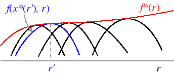
Here's an illustration of the math from lifted from the link above. The black and blue curves hold farmers's decisions fixed at different levels of $x$, optimized at each $r$  The $f^*(r)$ ( or $y^*$) we observe is the "upper envelope" of the all the blue and black curves with different, optimized levels of $x$.

Now, if $f^*(r)$ is highly nonlinear, and we are contemplating a very large change in climate, then adaptation will come into play. But even then it's probably not going to be a primary consideration.

I don't expect this basic insight, drilled into every economist during their first year of grad school (and even some undergraduates), will stop some economists from over-emphasizing adaptation.  But our own basic theory nevertheless indicates it is a small deal.  And it seems to me that the evidence so far bears this out just as clearly as the theory does.

Devise a better net-metering agreement for residential solar

A question for my undergraduate environmental economics students:

Navigate to http://www.uhero.hawaii.edu/news/view/274 and read about the costs and benefits of installing PV, from a household's perspective and from Hawaiian Electric's. Play around with the interactive calculator. Dick Rosenblum, the CEO of Hawaiian Electric, often complains about net metering agreements because homeowners get retail prices instead of wholesale prices for the energy their panels generate. (Also see this article by energy economist Severin Borenstein.) 

As the UHERO blog post points out, a side effect from current net metering agreements is that households over-install solar. As a result, they often pay a zero marginal price for electricity, which discourages conservation. 

Devise a different model for net metering agreements that can address both Dick Rosenblum's complaints and restore incentives for households with solar to conserve energy.

Feel free to help my students out by suggesting answers in the comment section ;-)

Pushing the limit of solar in Hawai'i

Sorry for the radio silence.  Way too much going on.

However, I am doing a little blogging for UHERO, focusing on Hawai'i's interesting electricity situation.  We have the highest electricity prices in the country, about 3.5 times those on the mainland.  That fact coupled with tax credits and a lot of sunshine has given us more solar penetration, by far, than anyplace in the country.  Most statistics you'll find tend to be a bit dated---there's more penetration here than most people know, and it's pushing the limit of our grid.

Anyhow, below are links to my first two posts about the situation.  More to come soon, I hope.

Is Monopoly a Barrier to Hawai'i's Ascent?

Why are Hawai'i's Electricity Prices So High?

Not fit to print, but why?

A brief follow up to my post the other day about the disasterous NY Times article by David Kocieniewski.

Flex Salmon and Jayson Lusk, among others, have written similar and more detailed pieces detailing Kocieniewski's reporting slight of hand.  I really thought this sort of thing was beneath the NY Times.  The editors there certainly deserve some of the blame.

Journalistic malfeasance aside, where is this attack coming from?  Why does Kocieniewski and NY Times go to such great lengths to attack two relatively innocuous academic economists?  Why do they seem to have a bee in their bonnet about commodity price speculation?

I don't know the answers to these questions.  But I'm wondering if momentum on financial regulatory reform may be a bit less innocent that Paul Krugman seems to think. Some might note that the Mike Konczal article that Krugman references mentions the heavy influence of Gary Gensler, chairman of the Commodity Futures Trading Commission.  I wonder if old powerful commodity interests may be an unlikely ally of Elizabeth Warren in the fight to regulate Wall Street banks more tightly.  The commodity groups aren't fans of regulation, and I doubt they share Warren's concern for consumers and market stability.  But presumably they don't like growing competition from Wall Street.  There would seem to be big private interests that favor financial reform.

Yes, I'm reading tea leaves here.  Does anyone have better insight?

NY Times attack by innuendo: Commodity price speculation edition

I've written a few times [e.g., 1, 2, 3, ] about commodity price speculation, arguing that speculation hasn't been the cause of volatility in recent years.  My views on this haven't changed, but I'm open to new arguments for why I and legions of other economists might be wrong. 

Overall, I haven't found this topic to be a very interesting, because those arguing that Wall Street caused the food price crisis, or caused oil prices to spike, really haven't presented any kind of logical argument.  All they do is point to the fact that Wall Street has gotten into the commodity game more than they have in the past.  But this isn't news and it falls far short of an explanation for how their trading activities are affecting prices. I haven't seen a serious study claiming a link, only magazine articles and opinion pieces, all thin on substance.  Professionally, I don't see this as interesting work.  This review lays things out pretty clearly.

I've been waiting for this issue to die.  But it seems there are political winds that won't let it.  Yesterday the New York Times came out with a new attack on academics, particularly Craig Pirrong and Scott Irwin.  These guys have been doing some consulting work, mainly for oil companies and the Chicago Mercantile Exchange.  These companies have also been giving money to their universities.  The documentary Inside Job is referenced (a great movie, by the way).  

There is a lot of innuendo in the story, and I do feel uncomfortable about academic economists getting cushy consulting contracts with big trading companies.  Still, the scale of what's mentioned seems tame relative to the kind of consulting gigs that seem commonplace in the economics realm of academia, or even the levels of corporate cash given to universities. 

The story is most notable for what it lacks: how, exactly, are the various companies distorting markets in a way that hurts consumers and or producers?  Inside Job describes the shady business of securities backed by stated-income mortgages, how Goldman Sachs was shorting the products it was selling to clients, etc.  We can see that there were shady business dealings and how they probably helped to fuel the real estate bubble.  So, where's the real underlying story in commodity market trading?

I don't think this story measures up to the New York Times' standard.  It's sad, because there might actually be a story here, but it would require a lot more legwork by Kocieniewski   That story, however, is probably a bit less salacious than what Kocieniewski was shooting for. My guess (I welcome challenges--I'm not sure about this) is that the  real story is a battle between old-school commodity groups (ADM, Cargill, and other so-called "majors" that both speculate and store commodities) and new competition from Wall Street, like JP Morgan Chase and Goldman Sachs.  I would further guess that some of the strangeness in commodity prices over recent years, like futures prices sometimes not converging to spot prices, is partly a refection of this changing marketplace.  Note, however, that the "strangeness" in pricing of which I speak has basically zero relevance to producer and consumer prices.  

My vague sense is that incompleteness in these markets---the fact that future contracts are only for certain months and certain delivery dates---procures a special advantage to the majors who control inventories at delivery points.  I'd further guess that Wall Street players are getting into commodities partly for diversification, and partly because they figure they can skim some the rents earned by the commodity players. 

Anyhow, I don't have all the details figured out.  It's something I started to pencil out once, but, like I said, I don't see this as especially useful for larger-scale questions about supply and demand, policy, climate change, etc. So I figure I've got better things to do.  

For the record, I've never had a consulting contract with commodity group or Wall Street firm.

Fixed Effects Infatuation

The fashionable thing to do in applied econometrics, going on 15 years or so, is to find a gigantic panel data set, come up with a cute question about whether some variable x causes another variable y, and test this hypothesis by running a regression of y on x plus a huge number of fixed effects to control for "unobserved heterogeneity" or deal with "omitted variable bias."  I've done a fair amount of work like this myself. The standard model is:

y_i,t = x_i,t + a_i + b_t + u_i,t

where a_i are fixed effects that span the cross section, b_t are fixed effects that span the time series, and u_i,t is the model error, which we hope is not associated with the causal variable x_i,t, once a_i

If you're really clever, you can find geographic or other kinds of groupings of individuals, like counties, and include group-by-year fixed effects:

y_i,t = x_i,t + a_i + b_g,t + u_i,t

The generalizable point of my lengthy post the other day on storage and agricultural impacts of climate change, was that this approach, while useful in some contexts, can have some big drawbacks. Increasingly, I fear applied econometricians misuse it.  They found their hammer and now everything is a nail.

What's wrong with fixed effects? 

A practical problem with fixed effects gone wild is that they generally purge the data set of most variation.  This may be useful if you hope to isolate some interesting localized variation that you can argue is exogenous.  But if the most interesting variation derives from a broader phenomenon, then there may be too little variation left over to identify an interesting effect.

A corollary to this point is that fixed effects tend to exaggerate attenuation bias of measurement errors since they will comprise a much larger share of the overall variation in x after fixed effects have been removed.

But there is a more fundamental problem.  To see this, take a step back and think generically about economics.  In economics, almost everything affects everything else, via prices and other kinds of costs and benefits.  Micro incentives affect choices, and those choices add up to affect prices, cost and benefits more broadly, and thus help to organize the ordinary business of life.  That's the essence of Adam's Smith's "invisible hand," supply and demand, and equilibrium theory, etc.  That insight, a unifying theoretical theme if there is one in economics, implies a fundamental connectedness of human activities over time and space.   It's not just that there are unobserved correlated factors; everything literally affects everything else.  On some level it's what connects us to ecologists, although some ecologists may be loath to admit an affinity with economics.

In contrast to the nature of economics, regression with fixed effects is a tool designed for experiments with repeated measures.  Heterogeneous observational units get different treatments, and they might be mutually affected by some outside factor, but the observational units don't affect each other.  They are, by assumption, siloed, at least with respect to consequences of the treatment (whatever your x is).  This design doesn't seem well suited to many kinds of observational data.

I'll put it another way.  Suppose your (hopefully) exogenous variable of choice is x, and x causes z, and then both x and z affect y.  Further, suppose the effects of x on z spill outside of the confines of your fixed-effects units.  Even if fixed effects don't purge all the variation in x, they may purge much of the path going from x to z and z to y, thereby biasing the reduced form link between x and y. In other words, fixed effects are endogenous.

None of this is to say that fixed effects, with careful account of correlated unobserved factors, can be very useful in many settings.  But the inferences we draw may be very limited.  And without care, we may draw conclusions that are very misleading. 

Can crop rotations cure dead zones?

It is now fairly well documented that much of the water quality problems leading to the infamous "dead zone" in the Gulf of Mexico (pictured above) come from fertilizer applications on corn. Fertilizer on corn is probably a big part of similar challenges in the Chesapeake Bay and Great Lakes.

This is a tough problem.  The Pigouvian solution---taxing fertilizer runoff, or possibly just fertilizer---would help.  But we can't forget that fertilizer is the main source of large crop productivity gains over the last 75 years, gains that have fed the world.  It's hard to see how even a large fertilizer tax would much reduce fertilizer applications on any given acre of corn.

However, one way to boost crop yields and reduce fertilizer applications is to rotate crops. Corn-soybean rotations are most ubiquitous, as soybean fixes nitrogen in the soil which reduces need for applications on subsequent corn plantings.  Rotation also reduces pest problems.  The yield boost on both crops is remarkable.  More rotation would mean less corn, and less fertilizer applied to remaining corn, at least in comparison to planting corn after corn, which still happens a fair amount.

I've got a new paper (actually, an old but newly revised paper), coauthored with Mike Livingston of USDA and Yue Zhang, a graduate student at NCSU, that might provide a useful take on this issue.  This paper has taken forever.  We've solved a fairly complex stochastic dynamic model that takes the variability of prices, yields and agronomic benefits of rotation into account. It's calibrated using the autoregressive properties of past prices and experimental plot data.  All of these stochastic/dynamics can matter for rotations. John Rust once told me that Bellman always thought crop rotations would be a great application for his recursive method of solving dynamic problems.

Here's the jist of what we found:

Always rotating, regardless of prices, is close to optimal, even though economically optimal planting may rotate much less frequently.  One implication is that reduced corn monoculture and fertilizer application rates might be implemented with modest incentive payments of  \$4 per acre or less, and quite possibly less than \$1 per acre.

In the past I've been skeptical that even a high fertilizer tax could have much influence on fertilizer use. But given low-cost substitutes like rotation, perhaps it wouldn't cost as much as some think to make substantial improvements in water quality.

Nathan Hendricks and coauthors have a somewhat different approach on the same issue (also see this paper).  It's hard to compare our models, but I gather they are saying roughly similar things.

Weather, storage and an old climate impact debate

This somewhat technical post is a belated followup to a comment I wrote with Tony Fisher, Michael Hanemann and Wolfram Schlenker, which was finally published last year in the American Economic Review.  I probably should have done this a long time ago, but I needed to do a little programming.  And I've basically been slammed nonstop.

First the back story:  The comment re-examines a paper by Deschanes and Greenstone (DG) that supposedly estimates a lower bound on the effects of climate change by relating county-level farm profits to weather.  They argue that year-to-year variation in weather is random---a fair proposition---and control for unobserved differences across counties using fixed effects.  This is all pretty standard technique.

The overarching argument was that with climate change, farmers could adapt (adjust their farming practices) in ways they cannot with weather, so the climate effect on farm profits would be more favorable than their estimated weather effect.

Now, bad physical outcomes in agriculture can actually be good for farmers' profits, since demand for most agricultural commodities is pretty steep: prices go up as quantities go down.  So, to control for the price effects they include year fixed effects.  And since farmers grow different crops in different parts of the country and there can be local price anomalies, they go further and use state-by-year fixed effects so as to squarely focus on quantity effects in all locations.

Our comment pointed out a few problems:  (1) there were some data errors like missing temperature data apparently coded with zeros and much of the Midwest and most of Iowa dropped from the sample without explanation; (2) in making climate predictions they applied state-level estimates to county-level baseline coefficients, in effect making climate predictions that regress to the state mean (e.g., Death Valley and Mt. Witney have different baselines but the same future); (3) all those fixed effects wash out over 99 percent of weather variation, leaving only data errors for estimation; (4) the standard errors didn't appropriately account for the panel nature of the spatially correlated errors.

These data and econometric issues got the most attention.  Correct these things and the results change a lot.  See the comment for details.

But, to our minds, there is a deeper problem with the whole approach.  Their measure of profits was really no such thing, at least not in an economic sense: it was reported sales minus a crude estimate of current expenditures.  The critical thing here is that farmers often do not sell what they produce.  About half the country's grain inventories are held on farm.  Farms also hold inventory in the form of capital and livestock, which can be held, divested or slaughtered.  Thus, effects of weather in one year may not show up in profits measured in that year.  And since inventories tend to be accumulated in plentiful times and divested in bad times, these inventory adjustments are going to be correlated with the weather and cause bias.

Although DG did not consider this point originally, they admitted it was a good one, but argued they had a simple solution: just include the lags of weather in the regression. When they attempted this, they found lagged weather was not significant, and thus concluded that this issue was unimportant.  This argument is presented in their reply to our comment.

We were skeptical about their proposed solution to the storage issue.  And so, one day long ago, I proposed to Michael Greenstone, that we test his proposed solution. We could solve a competitive storage model, assume farmers store as a competitive market would, and then simulate prices and quantities that vary randomly with the weather.  Then we could regress sales (consumption X price) against our constructed weather and lags of weather plus price controls. If the lags worked in this instance, where we knew the underlying physical structure, then it might work in reality.

Greenstone didn't like this idea, and we had limited space in the comment, so the storage stuff took a minimalist back seat. Hence this belated post.

So I recently coded a toy storage model in R, which is nice because anyone can download and run this thing  (R is free).  Also, this was part of a problem set I gave to my PhD students, so I had to do it anyway.

Here's the basic set up:

y    is production which varies randomly (like the weather).
q    is consumption, or what's clearly sold in a year.
p    is the market price, which varies inversely with q (the demand curve)
z    is the amount of the commodity on hand (y plus carryover from last year).

The point of the model is to figure out how much production to put in or take out of storage.  This requires numerical analysis (thus, the R code).  Dynamic equilibrium occurs when there is no arbitrage: where it's impossible to make money by storing more or storing less.

Once we've solved the model, which basically gives q, p as a function of z, we can simulate y with random draws and develop a path of q and p.  I chose a demand curve, interest rate and storage cost that can give rise to a fair amount of price variability and autocorrelation, which happens to fit the facts.  The code is here.

Now, given our simulated y, q and p, we might estimate:

(1)   q_t = a + b0  y_t + b1 y_{t-1} + b2 y_{t-2} + b3 y_{t-3} +  ... + error

(the ... means additional lags, as many as you like.  I use five.)

This expression makes sense to me, and might have been what DG had in mind: quantity in any one year is a function of this year's weather and a reasonable number past years, all of which affect today's output via storage.  For the regression to fully capture the true effect of weather, the sum of b# coefficients should be one.

Alternatively we might estimate:

(2)   p_t q_t = a + b0  y_t + b1 y_{t-1} + b2 y_{t-2} + b3 y_{t-3} +  ... + error

This is almost like DG's profit regression, as costs of production in this toy model are zero, so "profit" is just total sales.   But DG wanted to control for price effects in order to account for the pure weather effect on quantity, since the above relationship, the sum of the b# coefficients is likely negative.  So, to do something akin to DG within the context of this toy model we need to control for price.  This might be something like:

(3)  p_t q_t = a + b0  y_t + b1 y_{t-1} + b2 y_{t-2} + b3 y_{t-3} +  ... + c p_t + error

Or, if you want to be a little more careful, recognizing there is a nonlinear relationship, we might have a more flexible control for p_t, and use a polynomial. Note that we cannot used fixed effects like DG because this isn't a panel.  I'll come back to this later.  In any case, with better controls we get:
 
(4)   p_t q_t = a + b0  y_t + b1 y_{t-1} + b2 y_{t-2} + b3 y_{t-3} +  ... + c1 p_t  + c2 p_t^2 + c3 p_t^3 +  error

At this point you should be worrying about having p_t on both the right and left side.  More on this in a moment.  First, let's take a look at the results:

Equation 1:
            Estimate Std. Error t value Pr(>|t|)
(Intercept)     1.68       1.32    1.28     0.20
y               0.39       0.03   15.62     0.00
l.y             0.23       0.03    9.17     0.00
l2.y            0.10       0.03    3.83     0.00
l3.y            0.07       0.03    2.66     0.01
l4.y            0.07       0.03    2.69     0.01
l5.y            0.06       0.03    2.34     0.02

The sum of the y coefficients is 0.86.  I'm sure if you put in enough lags they would sum to 1. You shouldn't take the Std. Error or t-stats seriously for this or any of the other regressions, but that doesn't really matter for the points I want to make. Also, if you run the code, the exact results will differ because it will take a different random draw of y's, but the flavor will be the same.

Equation 2:
            Estimate Std. Error t value Pr(>|t|)
(Intercept)  4985.23     166.91   29.87        0
y             -72.15       3.19  -22.63        0
l.y           -43.67       3.20  -13.64        0
l2.y          -22.52       3.21   -7.03        0
l3.y          -15.61       3.21   -4.87        0
l4.y          -13.58       3.19   -4.26        0
l5.y          -12.26       3.19   -3.85        0

All the coefficients are negative.  As we expected, good physical outcomes for y mean bad news for profits, since prices fall through the floor.  If you know a little about the history of agriculture, this seems about right.  So, let's "control" for price.

Equation 3:
            Estimate Std. Error t value Pr(>|t|)
(Intercept)  2373.15     167.51   14.17        0
y             -28.12       2.91   -9.66        0
l.y           -17.72       2.10   -8.43        0
l2.y          -11.67       1.63   -7.17        0
l3.y           -8.07       1.57   -5.16        0
l4.y           -5.99       1.56   -3.84        0
l5.y           -5.68       1.54   -3.68        0
p               7.84       0.44   17.65        0

Oh, good, the coefficients are less negative.  But we still seem to have a problem.  So, let's improve our control for price by making it a 3rd order polynomial:

Equation 4:
            Estimate Std. Error       t value Pr(>|t|)
(Intercept)  1405.32          0  1.204123e+15     0.00
y               0.00          0  2.000000e-02     0.98
l.y             0.00          0  3.000000e-02     0.98
l2.y            0.00          0  6.200000e-01     0.53
l3.y            0.00          0 -3.200000e-01     0.75
l4.y            0.00          0 -9.500000e-01     0.34
l5.y            0.00          0 -2.410000e+00     0.02
poly(p, 3)1  2914.65          0  3.588634e+15     0.00
poly(p, 3)2  -716.53          0 -1.795882e+15     0.00
poly(p, 3)3     0.00          0  1.640000e+00     0.10

The y coefficients are now almost precisely zero. 

By DG's interpretation, we say that weather has no effect on profit outcomes and thus climate change is likely to have little influence on US agriculture.  Except in this simulation we know that in the underlying physical reality is that one unit of y ultimately has a one unit effect on the output.  DG's interpretation is clearly wrong.

What's going on here? 

The problem comes from an attempt to "control" for price.  Price, after all, is a key (the key?) consequence of the weather. Because storage theory predicts that prices incorporate all past production shocks, whether they are caused by weather or something else, in controlling for price, we remove all weather effects on quantities.  So, DG are ultimately mixing up cause and effect, in their case by using a zillion fixed effects. One should take care in adding "controls" that might actually be an effect, especially when you supposedly have a random source of variation.  David Freedman, the late statistician who famously critiqued regression analysis in the social sciences and provided inspiration to the modern empirical revolution in economics, often emphasized this point.

Now, some might argue that the above analysis is just a single crop, that it doesn't apply to DG's panel data. I'd argue that if you can't make it work in a simpler case, it's unlikely to work in a case that's more complicated.  More pointedly, this angle poses a catch 22 for the identification strategy: If  inclusion of state-by-year fixed effects does not absorb all historic weather shocks, then it implies that the weather shocks must have been crop- or substate-specific, in which case there is bias due to endogenous price movements even after the inclusion of these fixed effects. On the other hand, if enough fixed effects are included to account for all endogenous price movements, then lagged weather by definition does not add any additional information and should not be significant in the regression.  Prices are a sufficient statistic for all past and current shocks.

All of this is to show that the whole DG approach has problems.  However, I think the idea of using lagged weather is a good one if combined with a somewhat different approach.  We might, for example, relate all manner of endogenous outcomes (prices, quantities, and whatever else) to current and past weather. This is the correct  "reduced form."  From these relationships, combined with some minimalist economic structure, we might learn all kinds of interesting and useful things, and not just about climate change.   This observation, in my view, is the over-arching contribution of my new article with Wolfram Schlenker in the AER

I think there is a deeper lesson in this whole episode that gets at a broader conversation in the discipline about data-driven applied microeconomics over the last 20 years.  Following Angrist, Ashenfelter, Card and Krueger, among others, everyone's doing experiments and natural experiments.  A lot of this stuff has led to some interesting and useful discoveries.  And it's helped to weed out some applied econometric silliness.

Unfortunately, somewhere along the way, some folks lost sight of basic theory.   In many contexts we do need to attach our reduced forms to some theoretical structure in order to interpret them.  For example, bad weather causing profits to go up in agriculture actually makes sense, and indicates something bad for consumers and for society as a whole.

And in some contexts a little theory might help us remember what is and isn't exogenous.